Overview
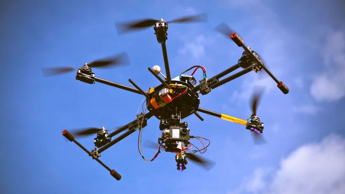
Small Uncrewed Aircraft Systems (sUAS) are aircraft that weigh less than 55 lbs and are used in agriculture, disaster response, logistics, climate research and wildlife monitoring, among many other things. Reliable, consistent navigation matters a lot for them.
Today the state of the art in navigation is GNSS, thanks to its wide availability and high accuracy. But GNSS is vulnerable to jamming, multipath effects and other weaknesses that come from relying on a satellite network, which has created real demand for autonomous navigation systems for sUAS.
Celestial navigation systems (CNS) are of particular interest because they work autonomously even when there are no terrain features. CNS fused with dead-reckoning inertial navigation (INS) has shown real promise for low-cost autonomous navigation.
This project looked at the feasibility of CNS/INS in sUAS given reasonable size, weight, power, cost, cooling and compatibility (SWaP-C3) constraints. It began with a literature survey of the state of the art, and then I worked to characterize an improved system that could reasonably be designed and manufactured in house.
Background and problem space
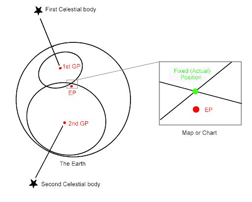
Celestial navigation has been used for centuries at sea. The process builds two Lines of Position (LOPs), where each line is all the points on Earth where an observer would measure the same angle to a celestial body, such as the azimuth or zenith of a star. Azimuth is the compass direction you face to see the object; zenith is the angle between the object and the point straight above you, so 0° means directly overhead and 90° means on the horizon.
Normally the LOP is built from the zenith angle, which makes it a circle around the object's Geographic Position, the point on Earth directly below it. With at least two LOPs you get two intersections, and they're usually far enough apart that you can pick the right one.
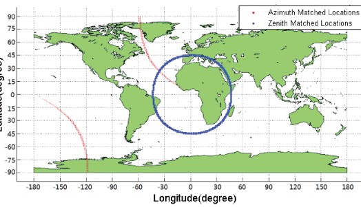
Celestial navigation is tricky for sUAS because they fly low, where atmospheric effects limit star visibility at night and nearly eliminate it during the day. So daytime solutions lean on the sun, and a single sun measurement only gives one LOP. My solution, written in MATLAB, uses two measurements of the sun instead of one: its zenith and its azimuth.
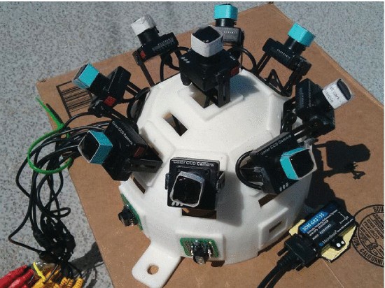
The hardware to support that can be cheap and easy to build: a hemispherical array of nine twenty-dollar CCD cameras and a two-hundred-dollar attitude heading reference system (AHRS), plus a mid-tier IMU at around two hundred dollars.
Improved algorithm
The program starts with a simulation module, where a set of positions over time are predefined and the solar azimuth and zenith values that would be measured at those positions are simulated. IMU data is simulated at the same time with a predefined MATLAB package.
The geolocation module that follows has a general outline similar to the reference paper (Liu et al., 2016), with one major difference coming from the simulated IMU data. The dead-reckoning IMU solution gives an initial guess of the sUAS's current location. A grid of coordinates is built around that guess with a preset latitude and longitude range and number of grid points. The theoretical solar azimuth and zenith at each point are calculated and compared with the "measured" values within a tolerance. The grid is cut down to only the points that pass, and the process repeats with the tolerance shrinking each time, until it reaches a target tolerance, ideally one set by instrumentation error.
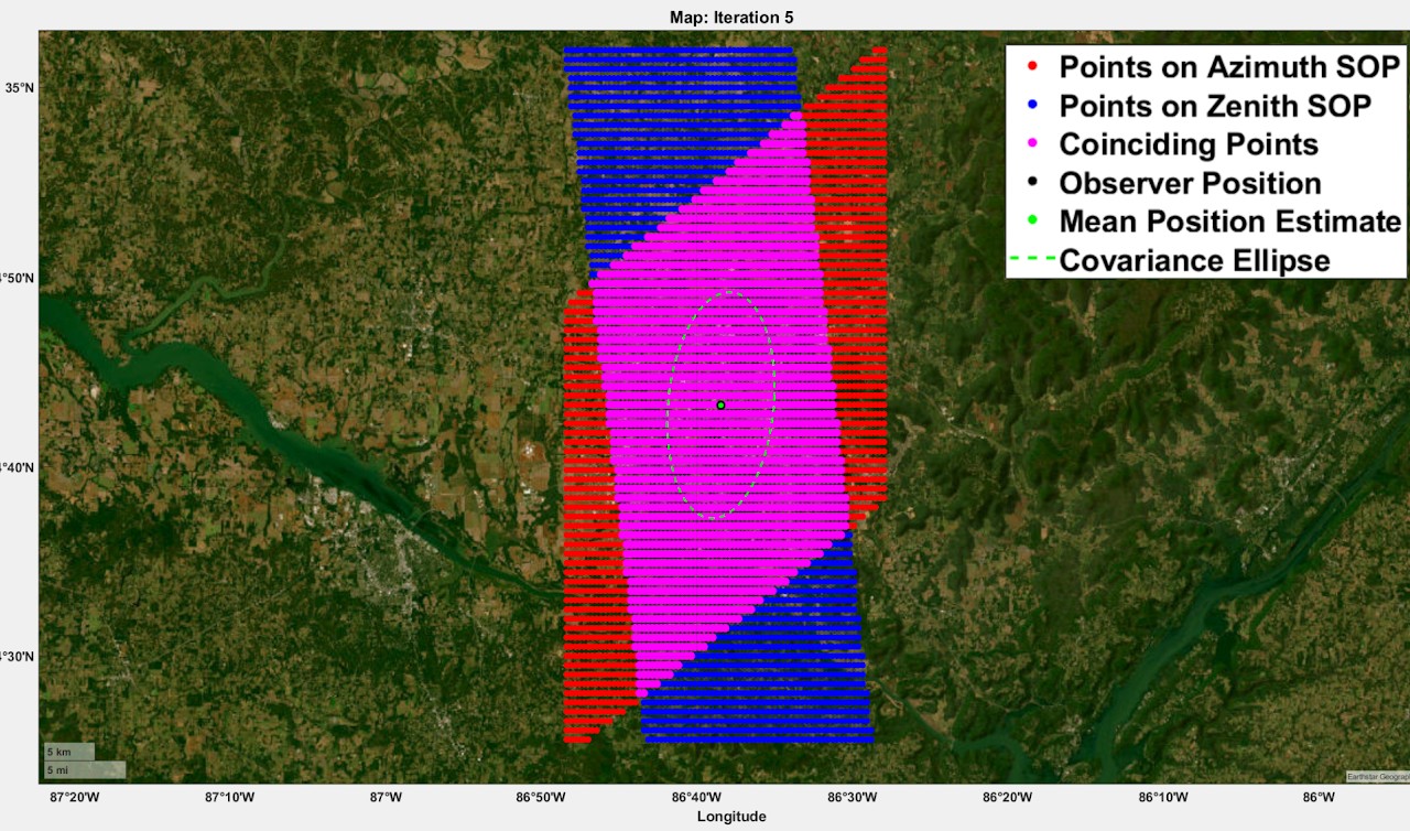
This avoids the computational burden of brute-force calculating the azimuth and zenith for every point on a high-resolution grid of the Earth. It takes a-priori IMU data to inform the next estimate and iterates to reach a satisfactory tolerance and grid size.
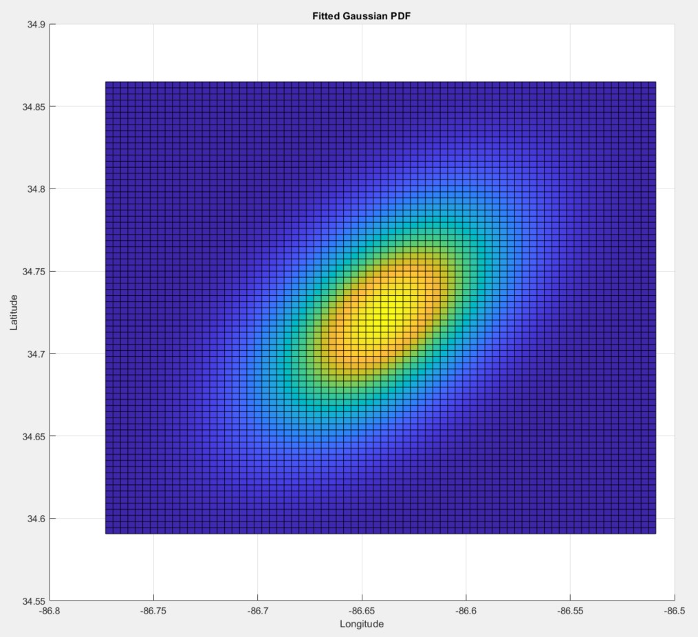
The program also models that each point on this grid of satisfactory locations is not equally probable, which turns out to be crucial. By modeling instrument error as a Gaussian and propagating those probabilities to the grid locations, I found that the solution can be fit to a 2D Gaussian, giving a solution in the form of a mean location and a stochastic covariance ellipse. That's a navigation solution that can be passed into state estimation filters, which would make the overall solution even more robust, and good enough for sUAS control algorithms.
Future developments
I got a navigation solution at about 5 Hz, up from 0.05 Hz, and I think there are steps that could improve it even more.
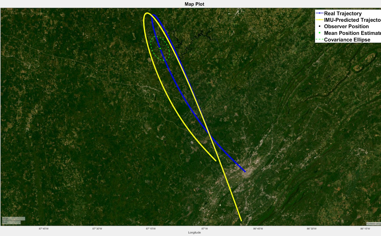
- Kalman filtering. A state estimation algorithm like a Kalman filter would give a more robust solution with lower uncertainty. It would also fix a problem in the current algorithm: as a trip goes on, the IMU estimate drifts away from the true trajectory, so the grid around the IMU estimate has to get bigger each iteration or trip duration has to be capped. A Kalman filter would fuse the IMU trajectory with the celestial solution and compensate for that drift.
- Real hardware. What's an algorithm without hardware to support it? Building and characterizing hardware would also show the real limits of the algorithm. For example, in some cases, cutting azimuth angle error by a factor of 10 makes the covariance ellipses hundreds of kilometers smaller.
Results and significance
A promising, reliable daytime celestial navigation algorithm built on a low-cost hardware setup. It shows potential for further improvement through Kalman filtering and is designed with that next step in mind. Simulation demonstrates the feasibility of autonomous celestial navigation in sUAS.
Skills used
- MATLAB
- Simulation and validation
- Hardware/software schematic development
- Project management
- Technical writing